This is a short guide to the basics of ampvis2, how to
load data, as well as a few basic visualisation functions using example
data. A complete explanation of all functions, their purpose, different
arguments and examples can be found in the Functions
tab.
Installation
Install ampvis2 as described on the home
page:
install.packages("remotes")
remotes::install_github("kasperskytte/ampvis2", Ncpus = 6)
Alternatively use the RStudio docker image with ampvis2 preinstalled as described on the home page.
Loading data
The first step is always to import some data by using the
amp_load function. The amp_load function is
quite flexible and auto-detects several different formats, including csv
or excel files, BIOM files, or even R objects directly. As a minimum,
you always need to import an abundance table with counts of OTU’s/ASV’s
per sample, the rest are optional, but any useful analysis involves
loading at least some sample metadata and taxonomy too. Refer to the amp_load
help page for details. A simple example would be:
library(ampvis2)
d <- amp_load(
  otutable = "path/to/otutable.csv",
  metadata = "path/to/samplemetadata.xlsx",
  taxonomy = "path/to/taxonomy.csv"
)
The amp_load function also supports importing data
directly from any of the commonly used amplicon processing pipelines
like QIIME, mothur, USEARCH, and DADA2. To import data in
the BIOM format from QIIME and
mothur (through the make.biom script), for
example, simply supply the path to the .biom file to the
otutable argument.
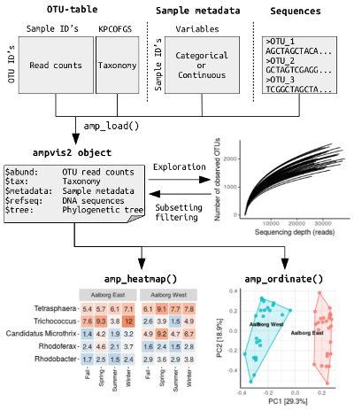
The data is then loaded and combined into a single
ampvis2 class object by the amp_load()
function, which makes the workflow a bit simpler as everything is
performed on a single object and can be manipulated by dedicated
functions. The data structure used in ampvis2 is inspired
by that of the phyloseq R
package, but instead of being an abstract S4 class object it’s a simple
list of data frames. The individual elements of the object
is otherwise the same and resembles that of a typical amplicon data set
(otutable, metadata, taxonomy, FASTA sequences, tree). Below is a simple
illustration of the data structure and typical workflow of
ampvis2:

Filtering and subsetting
With the ampvis2 package comes a large example data set
with 573 samples taken from the activated sludge from 55 Danish
Wastewater Treatment Plants in the period 2006-2013, which can be loaded
with data("MiDAS"). Simply typing the name of any ampvis2
object in the console will show a short summary of the data:
data("MiDAS")
MiDAS
## ampvis2 object with 5 elements.
## Summary of OTU table:
## Samples OTUs Total#Reads Min#Reads Max#Reads Median#Reads
## 658 14969 20890850 10480 46264 31800
## Avg#Reads
## 31749.01
##
## Assigned taxonomy:
## Kingdom Phylum Class Order Family
## 14969(100%) 14477(96.71%) 12737(85.09%) 11470(76.63%) 9841(65.74%)
## Genus Species
## 7380(49.3%) 28(0.19%)
##
## Metadata variables: 5
## SampleID, Plant, Date, Year, PeriodIf you have loaded the raw DNA sequences of the OTUs from a FASTA
file (with the fasta = argument) you can also get a short
summary by typing the name of the ampvis2 object followed by
$refseq:
MiDAS$refseq## 14969 DNA sequences in binary format stored in a list.
##
## Mean sequence length: 472.922
## Shortest sequence: 425
## Longest sequence: 525
##
## Labels:
## OTU_1
## OTU_2
## OTU_3
## OTU_4
## OTU_5
## OTU_6
## ...
##
## Base composition:
## a c g t
## 0.261 0.225 0.319 0.194
## (Total: 7.08 Mb)The loaded data can be subsetted based on variables in the metadata
using the amp_subset_samples() function, which can then be
stored as a new object and analysed separately:
MiDASsubset <- amp_subset_samples(
  MiDAS,
  Plant %in% c("Aalborg West", "Aalborg East")
)
## 590 samples and 5512 OTUs have been filtered
## Before: 658 samples and 14969 OTUs
## After: 68 samples and 9457 OTUsor for a more complex subset, you can subset based on two or more
variables using “&” to separate the conditions, or simply use the
function more than once. The “!” (logical NOT operator) can be thought
of as “except” and is useful to remove fx outliers. Furthermore, the
minreads = 10000 argument removes any sample(s) with total
amount of reads below the chosen threshold:
MiDASsubset <- amp_subset_samples(
  MiDAS,
  Plant %in% c("Aalborg West", "Aalborg East") & !SampleID %in% c("16SAMP-749"),
  minreads = 10000
)
## 591 samples and 5539 OTUs have been filtered
## Before: 658 samples and 14969 OTUs
## After: 67 samples and 9430 OTUsThe amp_subset_taxa() function instead subsets based on
the taxonomy, where you simply provide a vector with the taxa you are
interested in, separated by a comma:
MiDAS_Chloroflexi_Actinobacteria <- amp_subset_taxa(
  MiDAS,
  c("p__Chloroflexi", "p__Actinobacteria")
)
## 12245 OTUs have been filtered
## Before: 14969 OTUs
## After: 2724 OTUsThe taxonomic rank is indicated by fx “p__” for phylum and “g__” for
genus etc, followed by the name of the taxon (case-sensitive, first
letter almost always capital). To filter individual OTUs simply provide
the OTU name(s) as-is in a vector, fx c("OTU_1206").
Heatmap
All ampvis2 plots are generated using the ggplot2 package. You can change
the look of the plots to better suit your needs, add more layers to the
plots and use other ggplot2 functions in combination with ampvis plots
if needed. Refer to the ggplot2
documentation for more information. amp_heatmap() by
default aggregates to phylum level and shows the top 10 phyla, ordered
by mean read abundance across all samples:
amp_heatmap(
  MiDASsubset,
  group_by = "Plant"
)
## Warning: `aes_string()` was deprecated in ggplot2 3.0.0.
## ℹ Please use tidy evaluation idioms with `aes()`.
## ℹ See also `vignette("ggplot2-in-packages")` for more information.
## ℹ The deprecated feature was likely used in the ampvis2 package.
## Please report the issue at <https://github.com/kasperskytte/ampvis2/issues>.
## This warning is displayed once every 8 hours.
## Call `lifecycle::last_lifecycle_warnings()` to see where this warning was
## generated.## Warning: Using `size` aesthetic for lines was deprecated in ggplot2 3.4.0.
## ℹ Please use `linewidth` instead.
## ℹ The deprecated feature was likely used in the ampvis2 package.
## Please report the issue at <https://github.com/kasperskytte/ampvis2/issues>.
## This warning is displayed once every 8 hours.
## Call `lifecycle::last_lifecycle_warnings()` to see where this warning was
## generated.
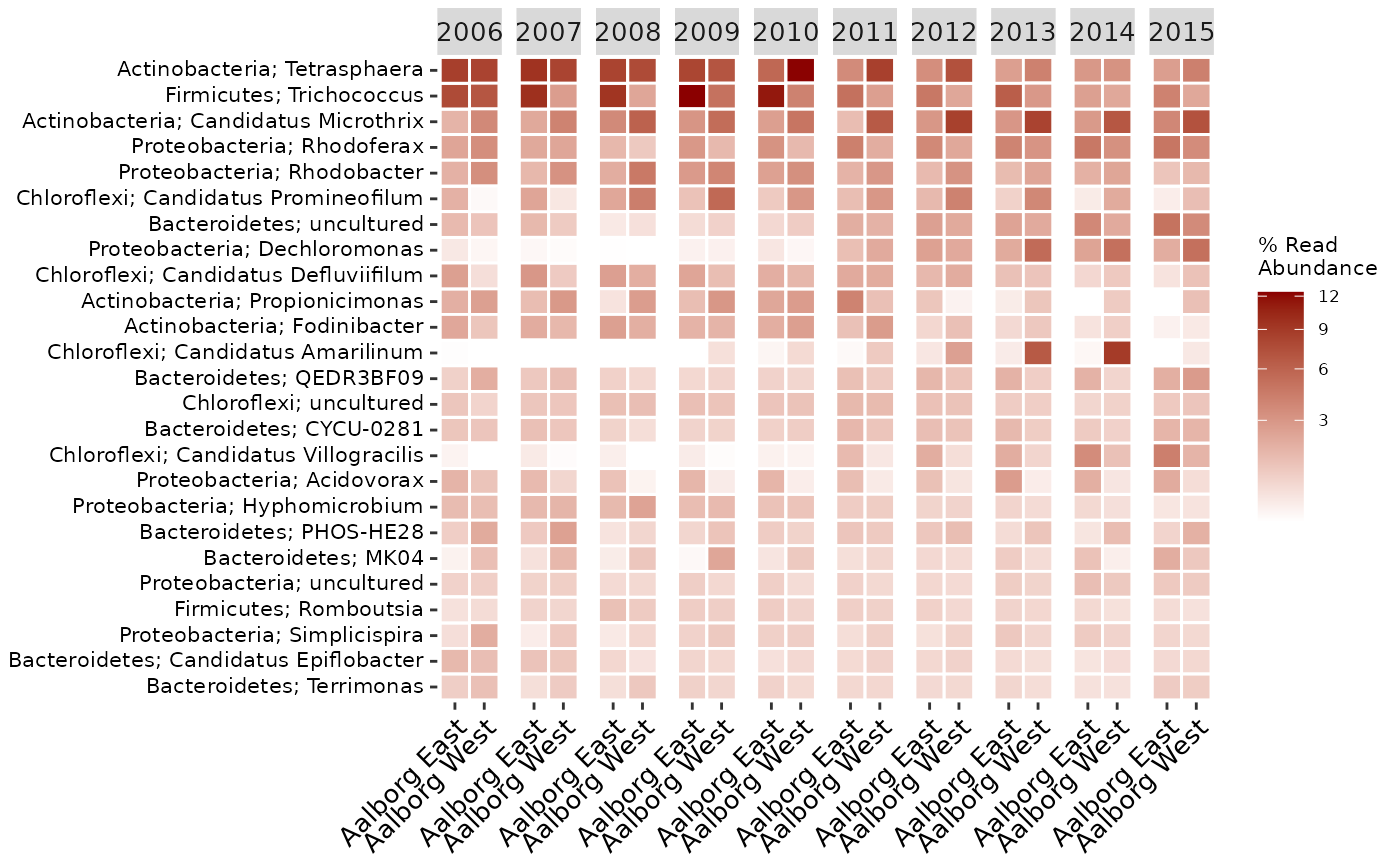
There are many arguments you can use to suit your needs, for a full list see the reference (click the function names to go to its reference page). For example, you can manually select the level at which to aggregate, how many to show, add additional higher level taxonomic information, group the samples differently by the metadata, hide the values, change the colors and scaling, and much more. You can also adjust the text labels for better readability or adjust the positioning of the legend (adjusting ggplot2 plots is always done with “+” after the actual ampvis2 function):
amp_heatmap(MiDASsubset,
            group_by = "Plant",
            facet_by = "Year",
            tax_aggregate = "Genus",
            tax_add = "Phylum",
            tax_show = 25,
            color_vector = c("white", "darkred"),
            plot_colorscale = "sqrt",
            plot_values = FALSE) +
  theme(axis.text.x = element_text(angle = 45, size=10, vjust = 1),
        axis.text.y = element_text(size=8),
        legend.position="right")
Boxplot
amp_boxplot() generates boxplots, again ordered by mean
read abundance across all samples:
amp_boxplot(MiDASsubset)
The arguments you can provide are similar to those used in
amp_heatmap() and other ampvis2 functions:
amp_boxplot(
  MiDASsubset,
  group_by = "Period",
  tax_show = 5,
  tax_add = "Phylum"
)
Ordination
The amp_ordinate() function has been expanded to support
7 different ordination methods, various data transformations and
interactive plots by using Plotly. By
default any OTU with an abundance no higher than 0.1% in any sample is
removed, which drastically improves the calculation time. You can of
course adjust this threshold manually by changing the
filter_species = 0.1 argument. Other than this, there are
only four main arguments that are involved in the actual calculations,
the rest are just various plotting features. These four are
type = "", transform = "",
distmeasure = "", and lastly constrain = ""
for constrained ordination (only used in Redundancy Analysis (RDA) or
Canonical Correspondence Analysis (CCA)).
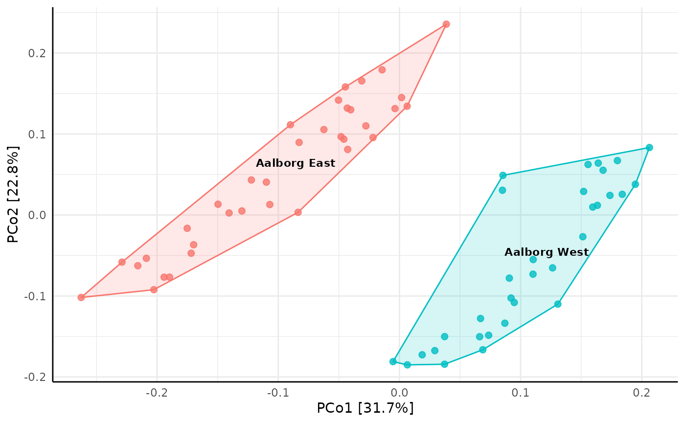
When analysing microbial community composition data it is recommended
to use the Hellinger transformation (see Legendre et al, 2001 or
Numerical
Ecology for details) for most types of ordination methods except the
distance-based ordination methods (Principal Coordinates Analysis (PCoA)
and non-Metric Multidimensional Scaling (nMDS)), where you also have to
select a distance measure manually by the distmeasure = ""
argument, for example Bray-Curtis dissimilarities:
amp_ordinate(
  MiDASsubset,
  type = "pcoa",
  distmeasure = "bray",
  sample_color_by = "Plant",
  sample_colorframe = TRUE,
  sample_colorframe_label = "Plant"
) +
  theme(legend.position = "blank")
It is also possible to track changes over time by setting the
sample_trajectory and sample_trajectory_group
arguments, to for example reveal temporal patterns per WWTP:
amp_ordinate(
  MiDASsubset,
  type = "pcoa",
  distmeasure = "bray",
  sample_color_by = "Plant",
  sample_colorframe_label = "Plant",
  sample_trajectory = "Date",
  sample_trajectory_group = "Plant"
)
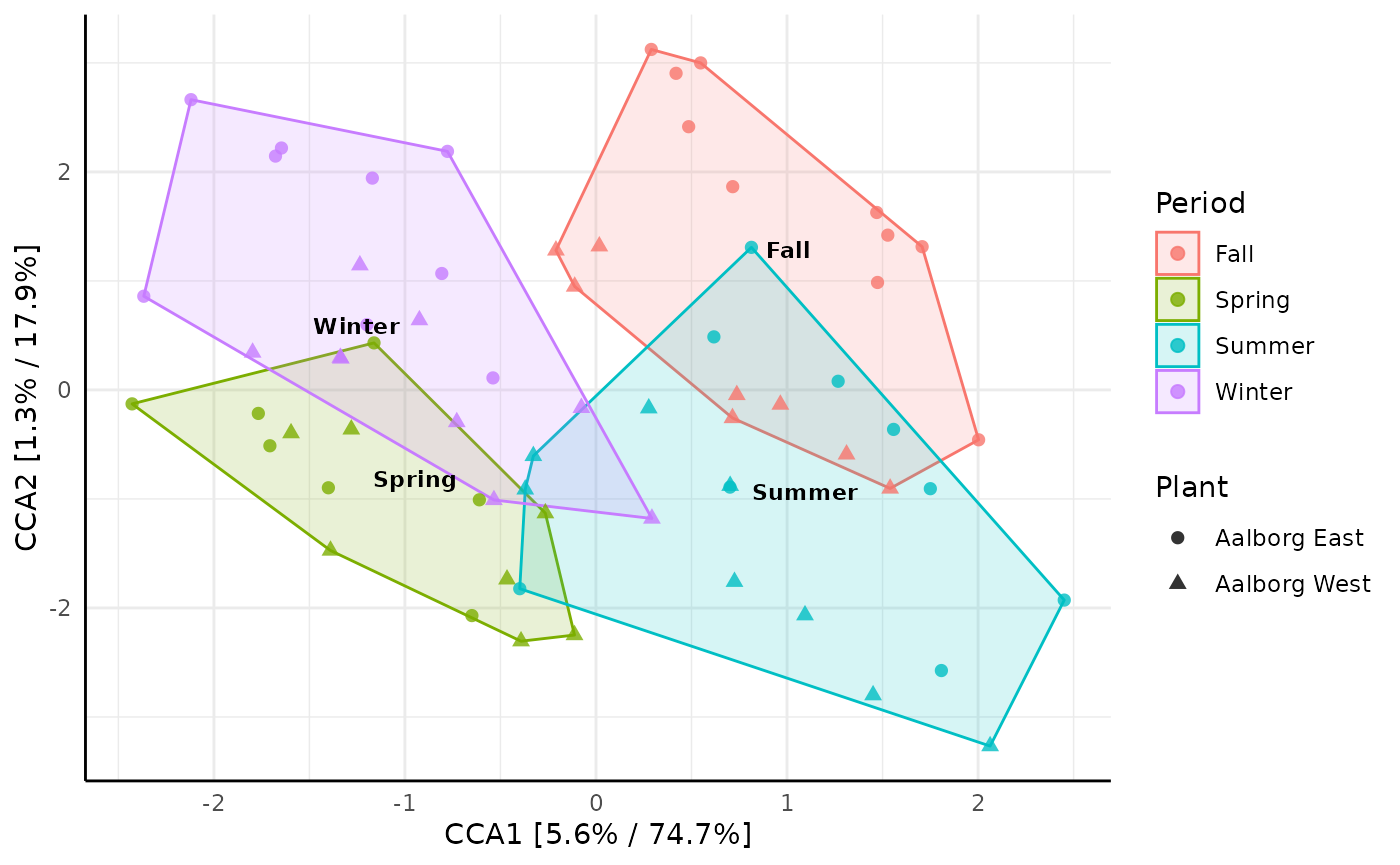
And lastly an example of constrained ordination by Canonical
Correspondence Analysis (CCA), which in this case reveals how samples
taken at different seasonal periods (constrain = "Period")
of the year can explain the data:
ordinationresult <- amp_ordinate(
  MiDASsubset,
  type = "CCA",
  constrain = "Period",
  transform = "Hellinger",
  sample_color_by = "Period",
  sample_shape_by = "Plant",
  sample_colorframe = TRUE,
  sample_colorframe_label = "Period",
  detailed_output = TRUE
)
ordinationresult$plot
Notice that the plot can be saved as a more detailed object
(detailed_output = TRUE), so additional details about the
ordination result can be obtained for evaluation, fx a screeplot by
ordinationresult$screeplot or some more raw data by
ordinationresult$model.
Read more
There are numerous other functions to try out as well as complete documentation for each function highlighted above. Go explore in the Functions tab.