2 Ordination in Microbial Ecology
To analyse the very large and complex multidimensional data obtained using NGS of sometimes hundreds of samples, each containing hundreds of different microorganisms, ordination is particularly suited because it can help reveal overall patterns in the data (Ramette, 2007). In essence, ordination seeks to reduce the dimensionality of a contingency table (objects in rows, descriptors in columns) into a few, usually 1-2, more important dimensions to ease interpretation, which makes it particularly suited for complex ecological data. Ordination methods are originally developed as largely heuristical approaches to solve particular ecological problems and most of the current ordination methods have been developed independently, but are similar in principle. Exactly when the first ordination method was developed is difficult to tell, but during the 1950s the term ‘ordination’ (from the German word ‘ordnung’, to order) were beginning to emerge to describe methods of classifying vegetation (Goodall, 1953), and several statistical approaches to answer specific ecological questions were proposed. For example the widely used Bray-Curtis measure was originally developed to examine the dominance behaviour of tree- and plant species in a forest in Southern Wisconsin (Bray & Curtis, 1957). Today, ordination methods have been used in countless ecological studies of the diversities of plants and animals, and have in the 21st century been readily applied in microbial ecology aswell (more than 7000 published studies) (Kuczynski et al., 2010; Ramette, 2007).
When performing ordination, \(n-1\) new, artificial dimensions are obtained through ‘dimensional yoga’, where \(n\) is the total number of objects, or samples in the case of ecology, each containing a part of the total inertia in the data, whether it be (co)variance, (dis)simililarity, or any other statistical property. The first axis will then display the most inertia, the second axis the second most, the third axis the third most etc, and plotting the first, usually two, axes can then reveal interesting patterns between the samples, simply by interpreting the distances between the points. It can be difficult for the human mind to grasp more than 3 dimensions (x,y,z), because this is something that only exists in math, and the complex math behind the scenes lies beyond the scope of this report. However, there are various different types of ordination, each suited for a particular purpose and understanding the key differences between them, which to use when, and why is important. The most commonly used ordination methods in microbial ecology will be described in the following.
2.1 Exploratory vs. Explanatory
The most commonly used ordination methods can generally be divided into two groups based on their purpose. The first group is the exploratory analyses, also known as unconstrained or indirect gradient analyses, which are suited for identifying global patterns between the objects (samples) based on the distribution or (dis)similarity of the values of multiple variables (species abundances) associated with them. The exploratory analyses do not take environmental variables (fx sample location, pH, temperature, nutrient concentrations etc, both qualitative or quantitative) into account and thus do not explain the revealed patterns directly. It is still possible to color or shape the points by known environmental variables (see Figure 2.1), however, but the scores (coordinates) on the ordination axes remain the same. The most commonly used exploratory methods in microbial ecology are Principal Components Analysis (PCA), non-Metric Multidimensional Scaling (nMDS), Principal Coordinates Analysis (PCoA/metric MDS) and Correspondence Analysis (CA) (Ramette, 2007).
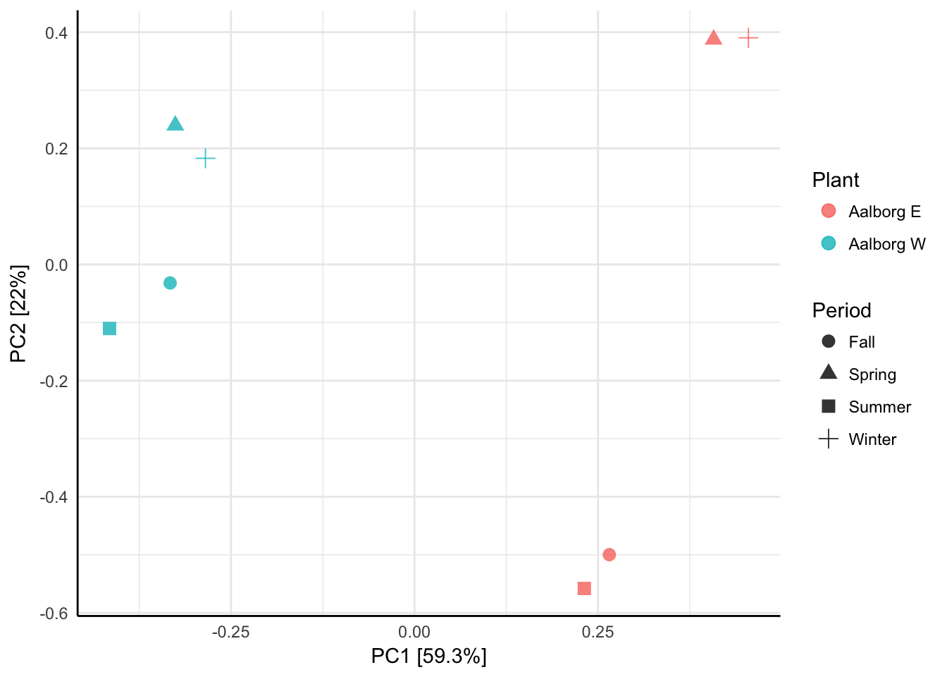
Figure 2.1: A minimal example of exploratory data analysis using Principal Components Analysis. 8 samples from two wastewater treatment plants, Aalborg East and Aalborg West have been analysed and the points have been shaped by when the samples were taken in 2012.
The second group is the explanatory analyses, also known as canonical, constrained or direct gradient analyses, which show only the variation in the data that can be explained by known environmental variables and not all the variation in the data as with unconstrained analysis. The response variables (species abundances) are thus considered to be the result of gradients along the environmental variables, or a combination of them. These gradients are called environmental gradients and the constrained ordination methods mainly differ in how they mathematically hypothesise the distribution of the response variables along the environmental gradient(s) to be, either linear or unimodal (P. Legendre & Legendre, 2012). Currently the two main constrained ordination methods used in microbial ecology are Redundancy Analysis (RDA) and Canonical Correspondence Analysis (CCA), which are considered extensions of Principal Component Analysis (PCA) and Correspondence Analysis (CA), respectively. RDA (and PCA for unconstrained analysis) is the optimal choice for purely linear distributions along the, preferably short, environmental gradient(s). CCA (and CA for unconstrained analysis) is the optimal choice for unimodal distributions along longer gradients where many double-zeros occur (more about double-zeros in Chapter 2.2), but in most cases CCA also performs well with short and linear gradients, it will just show a more qualitative representation of the samples (Braak & Prentice, 1988). Both RDA and CCA are eigenanalyses and calculate their constrained/canonical axes by introducing a linear combination of the response variables and the environmental variables as an additional step in the procedure. Otherwise the procedure is identical to that of PCA (when performing RDA) or CA (when performing CCA) (P. Legendre & Legendre, 2012). An overview of commonly used ordination methods in microbial ecology can be found in Table 2.1, and the kind of plots obtained when performing ordination is illustrated in Figure 2.2.
| Unconstrained analyses | Constrained analyses |
|---|---|
| Eigenanalysis-based | |
| Principal Components Analysis (PCA) | Redundancy Analysis (RDA) |
| Correspondence Analysis (CA) | Canonical Correspondence Analysis (CCA) |
| Distance-based | |
| non-metric Multidimensional Scaling (nMDS) | |
| Principal Coordinates Analysis (mMDS/PCoA) |
Figure 2.2: Schematic comparison of techniques that can be used to obtain unconstrained (a,b) or constrained (c-e) ordination biplots or triplots of species data tables. Source: (Legendre and Gallagher, 2001)
2.2 Niche theory and the double-zero problem
In reality there are often many, known or unknown, environmental variables affecting the presence of species and the gradient is then considered a complex environmental gradient. As niche theory states, species have ecological preferences and are present under a set of optimal environmental conditions, including the presence of other species (Hutchinson, 1957). The theory also predicts that species have unimodal distributions along environmental gradients, illustrated in Figure 2.3, so that they are found in greater abundances at some intervals along the major environmental gradients and gradually less present away from that optimal set of thriving conditions, ultimately absent (Whittaker, 1967). This has the consequence that community composition data typically contain many zeros, which can pose a problem for some ordination methods, specifically those using Euclidean distances like PCA and RDA (P. Legendre & Legendre, 2012).
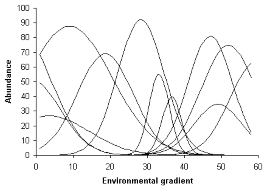
Figure 2.3: Species response (or abundance-) curves in most cases show a unimodal distribution along an environmental gradient. Adopted from (Whittaker, 1967)
The goal of using ordination is to represent patterns or differences between samples based on species abundances to draw ecologically meaningful conclusions about the sampling site(s) and their corresponding \(\beta\)- or \(\gamma\)-diversity (the diversity of local sites or whole regions of sites, respectively). The species abundances are considered to be response variables in the sense that they are indicators of their nearby environment. Variation in the environment is expected to be reflected in the relative productivities or abundances of the species (Whittaker, 1972). If a species is present at two sites, this means that the sites share conditions that are favorable for the species, indicating a similarity between the sites. On the contrary, if a species is present at one site and not the other, this indicates that the ecological conditions at the sites most likely are dissimilar. However, if a species is absent from both sites, it provides no valuable ecological information since both sites either have ecological conditions outside the niche of the species, and these conditions may be very similar or very different, or the niche has been occupied by another species prefering the same conditions. Including double zeros in the comparison of sites thus results in a higher similarity between the sites than there is ecologically, and this phenomena is called the double-zero problem (P. Legendre & Legendre, 2012). It is therefore important to consider whether there is relevant ecological information in double-zeros in the particular study, but in most cases it is preferable not to conclude anything ecologically about them and avoid including them in the analysis. This is called asymmetric analysis as double presences are treated differently than double absences and is done in practice when the distance coefficients between sites are computed, either implicitly or explicitly during ordination (P. Legendre & Legendre, 2012). Choosing the correct ordination method and, for some, also a distance measure therefore depends on whether this information is meaningful for the study. If linear ordination methods like Principal Components Analysis or Redundancy Analysis is used, then they should first be subjected to appropriate data transformation to correct for the problem and reflect the ecological differences more correctly (P. Legendre & Legendre, 2012).
2.3 Distance-based ordination
Fundamental to any ordination method is not only dimensional reduction, but more importantly also how it does so and how it displays and calculates distances between objects (sites) or variables (species). As stated in Table 2.1, ordination methods can be classified by whether they are distance-based or not, however they could just as well have been classified by whether they use a distance measure explicitly or implicitly to calculate distances, respectively (P. Legendre & Legendre, 2012). As such, eigenanalysis-based ordination methods use a distance measure of their own as part of their algorithm, while distance-based ordination can only be performed on a distance- or (dis)similarity matrix, which has to be calculated first using one of many distance- or (dis)similarity measures. When calculated, a symmetrical matrix is then obtained containing association coefficients between all pairs of sites. This gives the ecologist flexibility as to how it would be ecologically meaningful to represent the differences between sites or species, however it also implies the importance of knowing how to interpret the results based on the particular measure and choosing it wisely (more on distance measures in Chapter 2.3.3) (P. Legendre & Legendre, 2012). One of the disadvantages of using distance-based ordination, however, is that it is not possible to plot both sites and species together in a biplot, only the sites are plotted.
Currently the most used distance-based ordination methods are non-Metric Multidimensional Scaling (nMDS) and Principal Coordinates Analysis (PCoA), also called metric Multidimensional Scaling (mMDS) (Ramette, 2007). There is also Polar Ordination, which is rarely used and will not be detailed in the following.
2.3.1 Principal Coordinates Analysis
Principal Coordinates Analysis (PCoA) is very useful at exploring microbial ecology data because it can represent relationships between samples measured by any distance coefficient in Euclidean space (also called metric space, fx a Cartesian coordinate system). Therefore PCoA is also called metric Multidimensional Scaling, because it can represent the metric properties of the distance- or (dis)similarity matrix. When the distance measure is Euclidean, the results obtained by PCoA is identical to that of PCA (P. Legendre & Legendre, 2012).
Since the choice of distance measure directly influences the result, it has to be done with care. However, this is also one of the advantages of using PCoA because it is then possible to better deal with ecological problems like the double-zero problem while still using Euclidean mapping. The choice of distance measure also influences how the results are to be interpreted, as the original data is then a function of the chosen measure, which may be non-Euclidean, and does not always allow for a true representation in Euclidean space. Furthermore, it is possible to obtain negative eigenvalues of the resulting axes, especially when semi-metric or non-metric measures are used, and this should be corrected for if they occur on the main axes (ie the axes being plotted). The eigenvalue of an axis is an indication of its contribution of inertia to the total inertia in the data, which is therefore also obscured by the choice of distance measure and its value should not be directly refered to when performing PCoA (Ramette, 2007). PCoA is partly based on eigenanalysis, however it is more appropriate to classify it as a distance-based analysis, since it is highly dependent on the chosen distance measure.
2.3.2 non-Metric Multidimensional Scaling
Non-Metric Multidimensional Scaling (nMDS) is similar to PCoA in that it is also performed on a distance- or (dis)similarity matrix calculated using a suited measure. However, nMDS is different from PCoA on numerous aspects. PCA aswell as PCoA both try to maximise a linear correlation (of course dependent on the metric used in the case of PCoA) of species abundances along the environmental gradient, which will often result in an artifact called the horseshoe effect when the response variables are the result of a non-linear or long gradient (Podani & Miklós, 2002). This results in an arch shaped and incorrect pattern of the points leading to false conclusions. nMDS eliminates this by only preserving the ranked order of the distance coefficients between samples. As the name suggests, this makes the procedure non-metric, and the distances between points is therefore not to be interpreted numerically.
nMDS does not try to explain as much variation in the data as possible as with PCA or PCoA, but more the discontinuities in the data. It is a very robust technique that can handle missing values aswell as multiple data types at once. It has no distributional assumptions about the data compared to all other ordination methods, where the data is assumed to have for example linear or unimodal distributions as with PCA/RDA and CA/CCA, respectively. nMDS is therefore the ordination method of choice when the nature of the data is unknown (Buttigieg & Ramette, 2014; P. Legendre & Legendre, 2012).
nMDS is furthermore very different from other ordination methods by how it is computed. nMDS is an iterative procedure where the number of dimensions is chosen a priori (before analysis) and the algorithm tries to find a solution from either random starting points or from the results of a PCoA on the same data provided by the user. The solution is not unique as with all other ordination methods mentioned in this chapter and it is therefore recommended to run it multiple times to validate the result, preferably with different numbers of dimensions. During the algorithm, a stress value is calculated to express the goodness-of-fit of the solution and the procedure is repeated many times (20+ is not unusual) using the solution of the previous cycle as the starting point until the stress value does not change significantly and reach an acceptable, low value. A stress value is considered good when below 0.05, while below 0.1 is acceptable. A stress value above 0.2 is suspect and the results should not be trusted (Ramette, 2007). Generally choosing more dimensions will lower the stress value.
One of the major drawbacks of nMDS is that it is very computationally demanding. However, modern computers are getting increasingly more powerful, so this is less of a concern compared to the time during which the method was developed by the psychometricians Kruskal and Shepard at the Bell Telephone Labs in the 1960’s (Kruskal, 1964; Shepard, 1966).
2.3.3 Distance- and (dis)similarity measures
As mentioned, choosing a distance- or (dis)similarity measure that makes ecological sense is crucial for the analysis and subsequent interpretation of the ordination. A distance measure is basically a mathematical function with which to calculate distances between objects or variables in the data. There are many, many ways (60+) of calculating distance/association coefficients between objects and/or variables, however only the general concepts and most important differences will be covered in the following. For in-depth knowledge of how to calculate association coefficients using all metrics, semi-metrics, non-metrics and their exact formulae, refer to Chapter 7 in Numerical Ecology (P. Legendre & Legendre, 2012).
For association coefficients to be considered metric, the four properties listed below have to be satisfied. When this is true, the coefficient is called a distance coefficient or a metric coefficient, since it can be fully represented in Euclidean (metric) space (P. Legendre & Legendre, 2012):
The four metric properties
The distance between identical objects is \(0\), which is the lowest possible value:if \(a=b\), then \(D(a,b)=0\)
When the compared objects are not identical, the coefficient, and the distance, has a positive value:if \(a\neq b\), then \(D(a,b) > 0\)
Symmetry: the distance from A to B is the same as the distance from B to A:\(D(a,b) = D(b,a)\)
Triangle inequality: The sum of two sides of a triangle of points in Euclidean space is equal to or longer than the third side. In other words, the shortest distance between two points in Euclidean space is a straight line:\(D(a,b) + D(b,c) \geq D(a,c)\)
When one or more of the four properties are not satisfied, in most cases the fourth property (triangle inequality), the coefficients calculated are not considered to be metric coefficients, they are then termed semi-metric coefficients or (dis)similarity coefficients. When this is the case, distances cannot be ordinated (at least reliably) in Euclidean space and nMDS is the optimal ordination method. PCoA can also be used, but the eigenvalues of the axes plotted has to be first checked for negative eigenvalues. This is normally not the case for the main axes being plotted, however. Therefore considering whether the chosen measure is suitable for the ordination method used is important and the interpretation of the result should be done according to the logic of the chosen distance measure (P. Legendre & Legendre, 2012). Dissimilarity and similarity coefficients are often just termed similarity coefficients because it is straight forward to convert dissimilarity coefficients (D) to similarity coefficients (S) and vice versa: \(S=1-D\) (P. Legendre & Legendre, 2012). An overview of some of the most commonly used metrics in ecology is summed in Table 2.2
| Distance metrics | semi-Metrics | non-Metrics |
|---|---|---|
| Euclidean | Bray-Curtis (dissimilarity) | Kulczynski |
| Chord | Sørensen (dissimilarity) | |
| Mahalanobis | ||
| \(\chi^2\) (Pearson chi-square) | ||
| Manhattan | ||
| Canberra | ||
| Jaccard |
2.4 Eigenanalysis-based ordination
The eigenanalysis-based ordination methods have more specific purposes than the distance-based methods, because they are limited to represent the distances only by the capabilities of their implicit distance measure, where distance coefficients are not first calculated manually by the user. They all have a few things in common, however (P. Legendre & Legendre, 2012):
- There is always one unique solution with the particular data
- Each axis is an eigenvector associated with an eigenvalue expressing the axis’ contribution to the inertia in the data
- The axes are ranked by (and plotted by) the eigenvalues, highest to lowest
- The axes are orthogonal to eachother, thus uncorrelated and express their own ‘unique’ inertia
Normally, the two axes with the highest eigenvalues are plotted in a Cartesian coordinate system, where the highest eigenvalue axis is represented by the first axis and the second highest on the second axis. The most inertia in the data is therefore always represented by the first (x-)axis, which can, for example in the case of two distinct groups of sample points as seen with the example in Figure 2.1, often be interpreted as ‘between-group variation’. The secondmost inertia is expressed by the second (y-)axis and can then be interpreted as ‘within-group variation’ (P. Legendre & Legendre, 2012).
It is important to examine all eigenvalues obtained for each axis to confirm that the axes being plotted are significant and represent a large portion of the inertia in the data. To do this, a simple plot called a scree plot can be made where all axes are plotted on the first axis ordered by eigenvalue in decreasing order and their corresponding eigenvalue on the second axis, as illustrated in Figure 2.4. Optimally, the first two axes represent more than half of the inertia in the data and have high values compared to the rest of the axes, where the latter should make up a slightly decreasing, straight line. The worst case scenario is when all the values make up a nearly horizontal, straight line. In this case, the ordination is either failing at representing the inertia in the data and a different ordination method may be better suited for the data or there is simply no inertia to represent at all. The sum of all eigenvalues is always equal to the total inertia in the data and the corresponding eigenvalues of the axes plotted are often shown as a percentage of the total inertia on the axis labels. In the following, the remaining four ordination methods listed in Table 2.1 will be explained briefly (Ramette, 2007).
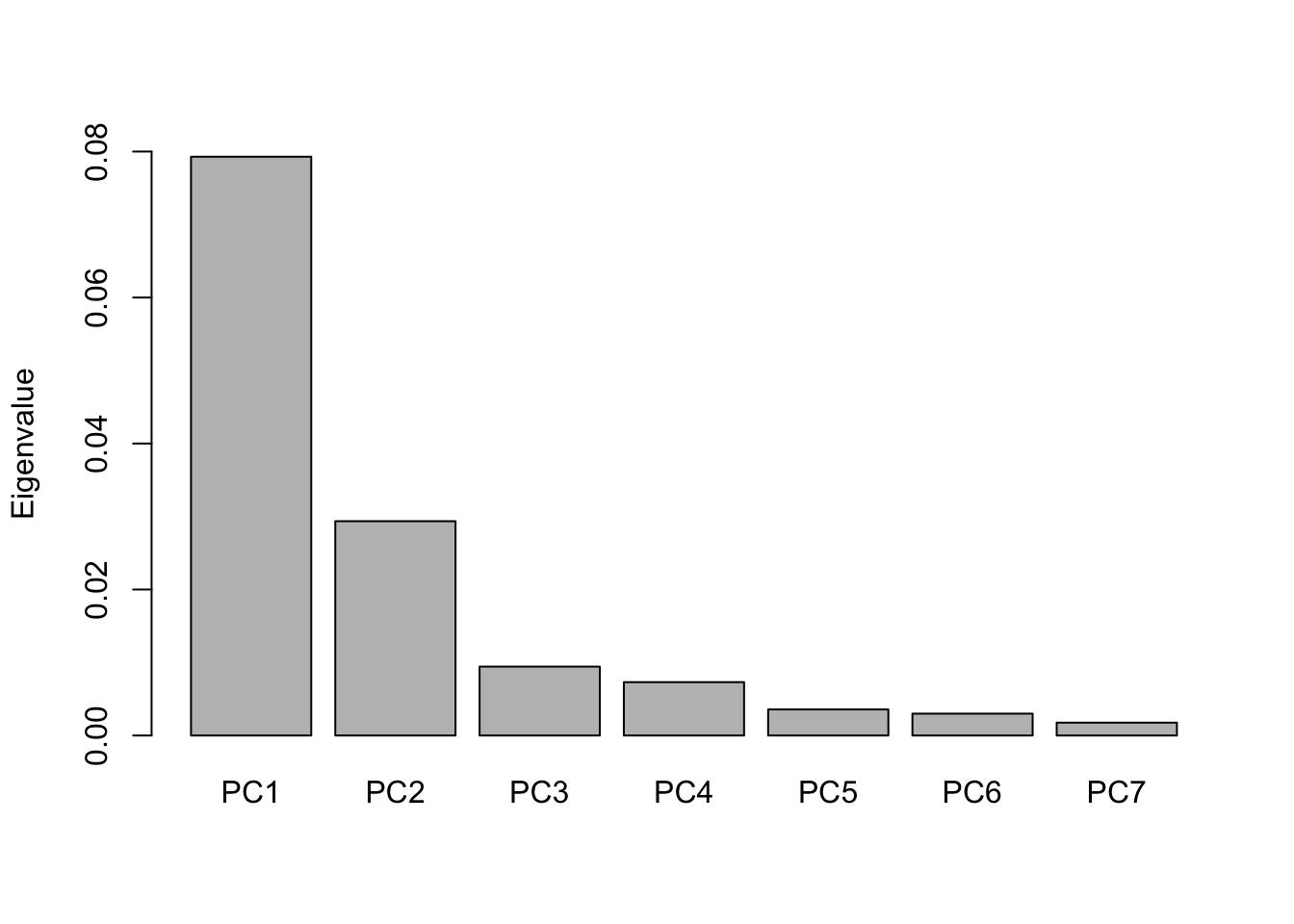
Figure 2.4: A scree plot of the eigenvalues of the 7 axes obtained from the PCA ordination seen in Figure 2.1.
2.4.1 Principal Components Analysis
Principal Component Analysis (PCA) is the oldest ordination method and still also the most used, perhaps due to its simplicity (Ramette, 2007). It has its roots all the way back to 1901 when Karl Pearson explained how to represent objects by the ‘best-fitting’ line or plane (Pearson, 1901). The simplest example of dimensional reduction is the representation of 2-dimensional data in 1 dimension, which is normally called linear regression. It is simply a straight line, drawn through the centroid of the data, see Figure 2.5.
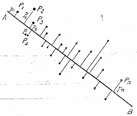
Figure 2.5: The main structure of two-dimensional data can often be described in one dimension by positions on a straight line. Adopted from (Pearson, 1901)
Pearson described how this is done mathematically, which formed the concepts of how to describe the overall structure of complex data. In 1933, Harold Hotelling (Hotelling, 1933) applied the concepts on multidimensional data and explained how to represent the data by its principal components, which in turn formed the fundamentals of PCA.
The goal of PCA is simple: express the maximum amount of variation in the data. This is done by generating new, synthetic axes, which are synonymous to eigenvectors, where the first axis is alligned so that it represents the most inertia in the data, where inertia in the case of PCA is specifically: variance. PCA is therefore considered more of a quantitative ordination method, as it excels at highlighting differences between samples based on numerical differences in species abundances and is most reliable when the same species are present in most or all of the samples (P. Legendre & Legendre, 2012). As mentioned in Chapter 2.2, this is rarely the case with ecological data, and the double-zero problem thus has a major impact on the results obtained by PCA, questioning its usefulnes without appropriate data transformation. Of course, this is not a problem when analysing \(\alpha\)-diversities (the diversity of a single sample) since there will be no zero-abundances (P. Legendre & Legendre, 2012).
PCA is a linear method because it represents the linear correlation or covariance of species abundances between samples using Euclidean distances. Both the sample scores (points) and species scores (arrows) are usually plotted together to form a biplot (refer to Figure 2.2), where arrows indicate the linear gradients of species abundances and the relative right-angle projections of the samples onto the arrows then approximate their corresponding abundance of the particular species. This makes PCA suited to answer questions like for example: “How are samples different in terms of the abundances of species X and Y?”, where X and Y are also among the most abundant species (Ramette, 2007).
Fundamental to PCA (and Redundancy Analysis) is the Euclidean distance, which is calculated by the following formula, equivalent to the pythagorean theorem:
The euclidean distance \[\begin{equation} D_{Euclidean}(x_1,x_2)=\sqrt{\sum_{j=1}^p\left(y_{1j}-y_{2j}\right)^2} \label{eq:eucdist} \end{equation}\]where \(Y=[y_{ij}]\) is a species abundance table of the size \((n{\times}p)\) with sites (rows) \(i=[1...n]\) and species (columns) \(j=[1...p]\). (P. Legendre & Gallagher, 2001)
2.4.2 Redundancy Analysis
To answer a question like: “How do species abundances correlate with a measured carbon source concentration?”, PCA would be insufficient. To answer that question, Redundancy Analysis (RDA) is the perfect choice. RDA is considered an extension of PCA, or the constrained version of PCA, which can directly explain the observed patterns based on known environmental variables. This is done by making a linear combination of the species abundance matrix and a matrix containing information about one or several known environmental variables. These variables are then hypothesised to be able to explain a portion of the observed variance in the data and the resulting constrained axes are plotted. Just as with unconstrained ordination, the two axes with the highest eigenvalues are plotted and their contribution to the total variance in the data is usually indicated on the axis labels to give an indication of the significance of the constrained variable(s) (Buttigieg & Ramette, 2014). When doing constrained analysis, both with RDA and CCA (Chapter 2.4.3), a plot with not only sites and species are made, but also environmental vectors are plotted together in one plot called a triplot (refer to Figure 2.2). This is a very convenient way to visualise all three types of information at once to easily draw ecological conclusions about the sites sampled.
Because RDA is based on Euclidean distances just like PCA, it is only suited for the analysis of short, linear environmental gradients with few or no species absences, which can limit its use in ecology (Minchin, 1987; Ramette, 2007).
2.4.3 Correspondence Analysis and Canonical Correspondence Analysis
Perhaps the most appropriate ordination method for ecological data is Correspondence Analysis (CA) because it represents the differences between sites hypothesising a unimodal distribution, which fits the species niche theory well, as discussed in Chapter 2.2. As the name suggests, CA tries to represent the correspondence between samples and species by showing how “this species correspond to that site”. The relative positions between species points and samples points are then to be interpreted as probabilities of the samples to contain the particular species nearby (P. Legendre & Legendre, 2012). CA is thus considered more of a qualitative representation of the data and is based on the Pearson chi-squared statistic of the form \(\chi^2 = \sum\frac{(observed-expected)^2}{expected}\).
CA is developed by several authors independently (though mainly the work of Braak & Prentice (1988) and Hill (1973) is credited) and has several different names, for example contingency table analysis, reciprocal averaging, weighted averaging, dual scaling or homogeneity analysis. Fundamentally, CA calculates the weighted averages of the species as defined by the \(\chi^2\)-distance described below, where the weights are, with community composition data, specifically species abundances (Braak & Prentice, 1988; P. Legendre & Legendre, 2012). This has the advantage that absent species in the samples have exactly zero weight and therefore do not result in higher similarities between the samples. It also means that species abundances contribute to the calculated distances, but only to a lesser degree because they are calculated relative to the average abundances and therefore do not influence the results as much as with the Euclidean-based ordination methods (PCA/RDA). This has the consequence that low abundant species may have an unduly high influence on the results, because the abundances of common species contribute less to the calculated distance compared to low abundant species, which are often numerous (P. Legendre & Gallagher, 2001). With CA, and CCA, it can therefore be relevant to give less weight to the low abundant species if needed.
The eigenvalues of the axes in CA (and CCA) are not equivalent to those in PCA/RDA and should not be interpreted as variance but as correlation coefficients, which reflects the degree of correspondence between the samples and species (Buttigieg & Ramette, 2014). Canonical Correspondence Analysis (CCA) will not be described further as it is simply the constrained version of CA in the exact same way as RDA is the constrained version of PCA, where a linear combination of the species abundance matrix and the explanatory variables are calculated as an additional step in the procedure, otherwise CA and CCA are the same. Fundamental to CA and CCA is the \(\chi^2\)-distance, which is calculated by the following formula:
The \(\chi^2\)-distance \[\begin{equation} D_{\chi^2}(x_1,x_2)=\sqrt{y_{++}}\sqrt{\sum_{j=1}^p\frac{1}{y_{+j}}\left(\frac{y_{1j}}{y_{1+}}-\frac{y_{2j}}{y_{2+}}\right)^2} \label{eq:chidist} \end{equation}\]where \(Y=[y_{ij}]\) is a species abundance table of the size \((n{\times}p)\) with sites (rows) \(i=[1...n]\) and species (columns) \(j=[1...p]\), with row sums \(y_{i+}\), column sums \(y_{+j}\) and total sum \(y_{++}\). (P. Legendre & Gallagher, 2001)