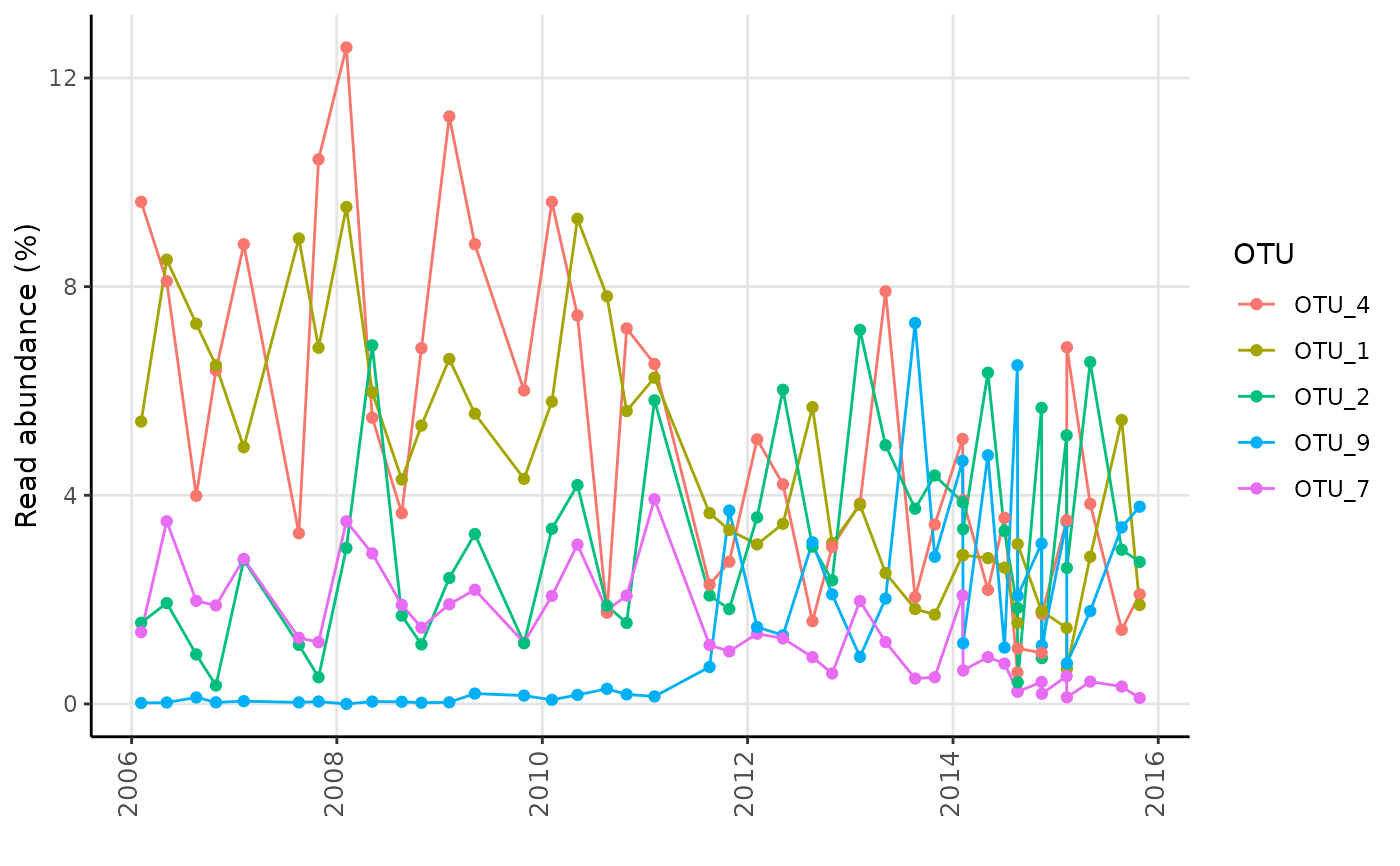
Generates a timeseries plot showing relative read abundances over time.
amp_timeseries(
  data,
  time_variable = NULL,
  group_by = NULL,
  tax_aggregate = "OTU",
  tax_add = NULL,
  tax_show = 5,
  tax_class = NULL,
  tax_empty = "best",
  split = FALSE,
  scales = "free_y",
  normalise = TRUE,
  plotly = FALSE,
  ...
)

amp_time_series(
  data,
  time_variable = NULL,
  group_by = NULL,
  tax_aggregate = "OTU",
  tax_add = NULL,
  tax_show = 5,
  tax_class = NULL,
  tax_empty = "best",
  split = FALSE,
  scales = "free_y",
  normalise = TRUE,
  plotly = FALSE,
  ...
)
Arguments
- data
(required) Data list as loaded with
amp_load.- time_variable
(required) The name of the column in the metadata containing the time variables, e.g.
"Date". Must be directly compatible withas_dateand preferably of the form"yyyy-mm-dd"or"%Y-%m-%d".- group_by
Group the samples by a variable in the metadata.
- tax_aggregate
The taxonomic level to aggregate the OTUs. (default:
"OTU")- tax_add
Additional taxonomic level(s) to display, e.g.
"Phylum". (default:"none")- tax_show
The number of taxa to show, or a vector of taxa names. (default:
6)- tax_class
Converts a specific phylum to class level instead, e.g.
"p__Proteobacteria".- tax_empty
How to show OTUs without taxonomic information. One of the following:
"remove": Remove OTUs without taxonomic information."best": (default) Use the best classification possible."OTU": Display the OTU name.
- split
Split the plot into subplots of each taxa. (default:
FALSE)- scales
If
split = TRUE, should the axis scales of each subplot be fixed (fixed), free ("free"), or free in one dimension ("free_x"or"free_y")? (default:"fixed")- normalise
(logical) Transform the OTU read counts to be in percent per sample. (default:
TRUE)- plotly
(logical) Returns an interactive plot instead. (default:
FALSE)- ...
Additional arguments passed to
as_dateto make the time_variable compatible with the timeseries plot, fx theformatortzarguments, see?as_date.
Value
A ggplot2 object.
Preserving relative abundances in a subset of larger data
See ?amp_filter_samples or the ampvis2 FAQ.
See also
Examples
# Load example data
data("AalborgWWTPs")

# Timeseries of the 5 most abundant OTUs based on the "Date" column
amp_timeseries(AalborgWWTPs,
  time_variable = "Date",
  tax_aggregate = "OTU"
)
#>
#> Attaching package: ‘lubridate’
#> The following objects are masked from ‘package:base’:
#>
#>     date, intersect, setdiff, union
#> Warning: Duplicate dates in column Date, displaying the average for each date.
#>  Consider grouping dates using the group_by argument or subset the data using amp_filter_samples.


# As the above warning suggests, there are more than one sample per date in the data,
# in this case one from Aalborg East and one from Aalborg West. The average of the
# two samples is then shown per date. In such case it is then recommended to either
# subset the data, or group the samples by setting group_by = "" and split by tax_aggregate
# by setting split = TRUE:
amp_timeseries(AalborgWWTPs,
  time_variable = "Date",
  group_by = "Plant",
  split = TRUE,
  scales = "free_y",
  tax_show = 9,
  tax_aggregate = "Genus",
  tax_add = "Phylum"
)
# As the above warning suggests, there are more than one sample per date in the data,
# in this case one from Aalborg East and one from Aalborg West. The average of the
# two samples is then shown per date. In such case it is then recommended to either
# subset the data, or group the samples by setting group_by = "" and split by tax_aggregate
# by setting split = TRUE:
amp_timeseries(AalborgWWTPs,
time_variable = "Date",
group_by = "Plant",
split = TRUE,
scales = "free_y",
tax_show = 9,
tax_aggregate = "Genus",
tax_add = "Phylum"
)
